The Estimated Accuracy Numbers (EAN) are representative of the signature of different error signals on the products, including both uncorrelated (i.e., noise) and correlated (spatial and temporal scale) error signals.
key numbers of the observable wavelengths with the DUACS L3 5Hz and 1Hz products are given in the QUID document.
Uncorrelated errors or measurement noise and mesoscale observability
The measurement noise is mainly induced by instrumental (altimeter) measurement errors. It can be mitigated with specific processings and corections (e.g. Moreau et al., 2021; Tran et al., 2021) and thus strongly depend on the altimeter data processing and standards applied.
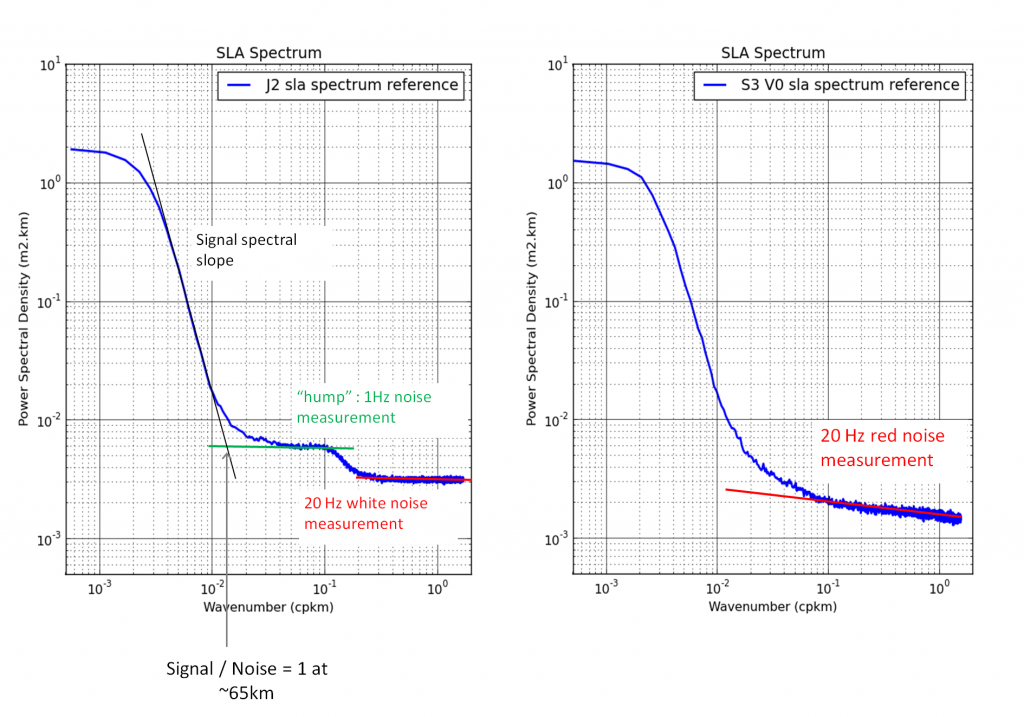
The measurement noise is quantified by an analysis of the wavenumber spectra of the SLA (figure 1). Indeed, the uncorrelated measurement error is the noise level estimated as the mean value of energy at high wavenumbers (wavelengths smaller than ~5 km).It have the same tendances of the the instrumental white-noise linked to the Surface Wave Height. For the conventional radar altimeter measurement (e.g., LRM mode), the inhomogeneity of the sea state within the altimeter footprint also induces an error visible as a “hump” in the wavenumber spectra of the SLA. As it also limits the short wavelenght signal observation, the noise error associated to the conventional radar measurement is estimated using the wavelenght range of the hump. The full understanding of this hump of spectral energy Dibarboure et al., (2014) remains to be achieved. This issue is strongly linked with the development of new retracking, new editing strategy or new technology. For the SAR measurement, part of the high frequency signal is characterized by a correlated signal (figure 1). This signal still needs to be fully explained. At this time, it is considered as an additional unknown signal that is assumed to be a “red noise” error considering the ocean geostrophic signal.
The mean 1 Hz and 5 Hz measurement noise observed for the different altimeters is summarized in Table 3 section I.3 in QUID. The product SEALEVEL_GLO_PHY_NOISE_L4_STATIC_008_033 gives the normalized spatial variation of this noise, mainly correlated with high/low wave heights areas. It was defined using one year of SARAL/Altika measurement and following the spectral decomposition methodology described in Vergara et al. (2019). Note that this product gives an annual mean status of the noise level. It does not take into account the temporal variability of the wave height that modulate the noise, as discussed in Dufau et al., 2016 and Vergara et al. (2019). The spatial distribution of the noise level for each mission is retrieved using the global mean noise amplitude given in Table 3 section I.3 in QUID (see PUM for details). Figure 2 shows the example for the Jason-3 mission with 1 Hz sampling.
The presence of measurement noise on along-track products limits the observability of the shorter mesoscales. The SLA power spectrum density analysis was used to determine the wavelength where signal and error are on the same order of magnitude (figure 1). It represents the minimum wavelength associated with the dynamical structures that altimetry would statistically be able to observe with a signal-to-noise ratio greater than 1. This wavelength has been found to be variable in space and time (Dufau et al., 2016; Vergara et al., 2022).
The mean observable wavelength with the conventional 1 Hz measurement was found to be nearly 65 km. It was defined with a single year of Jason-2 measurements over the global ocean, excluding latitudes between 20°S and 20°N (mainly due to the limit of the underlying surface quasi-geostrophic turbulence in these areas).
The mean observable wavelength over the Europe area, observed with the regional Europe L3 5 Hz SLA, was found to range between 55 km (Jason-3) to 40 km (S6A) (Table 10 section I.3 in QUID). These last values were obtained taking into account the unbalanced motion signal as described in Vergara et al. (2022), and using only few months of measurements (April-June2022).
The mean observable wavelength over the global ocean, observed with the Global L3 5 Hz SLA, is in the same order as the one observed over the European area (Table 10 section I.3 in QUID). However, a clear regional pattern is underscored, as shown in Figure 1 in Along-track (L3) products generation, and locally the observable wavelength range between ~20 km (Sentinel-6A) and ~more than 100 km (HY2B). These values were obtained over the period covering October 2022-July 2023, considering only the dynamical balanced motion and the measurement noise as described in Dufau et al., 2016.
The Observable wavelength will evolve in the future, depending on advances in the determination method and the availability of longer data series.
a)

b)
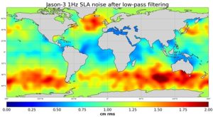
Figure 2: The 1 Hz measurement noise observed along Jason-3 tracks before (a) and after (b) along-track filtering processing. Note that the scales are different in each panel; unit : root mean square (cm rms).
Errors at climatic scales
In the framework of the ESA SL-CCI project, the altimeter measurement errors at climatic scales have been estimated using the Topex/Poseidon, Jason-1, Jason-2 and Jason-3 missions. Details on the error budget estimation at climatic scale can be found in Ablain et al.,( 2019) and Guérou et al., (2022). Results are summarized in Table 3 section I.3 in QUID.
All the parameters/algorithms involved in the altimeter measurement processing can induce errors at climatic scales. However, some parameters contribute more strongly than others. The largest sources of errors for Global Mean Sea Level trend estimation have been identified. They concern i) the radiometer wet tropospheric correction with a drift uncertainty in the range of 0.2~0.3 mm/yr Legeais et al., (2014), ii) the orbit error Couhert et al., (2015) and iii) the altimeter parameters (range, sigma-0, SWH) instabilities Ablain et al., (2012), with additional uncertainty of the order of 0.1 mm/yr over the whole altimeter period, and slightly more over the first decade (1993-2002; Ablain, (2013). Errors of multi-mission calibration (see §Systeme – Homogeneization ans cross-calibration) also contribute to the Global Mean Sea Level (GMSL) trend error of about 0.15 mm/yr over the 1993-2010 period Zawadzki and Ablain, (2016). All sources of errors described above also have an impact at the inter annual time scale (< 5 years) close to 2 mm over a 2-5 years period.
The regional sea level trend uncertainty has an average estimate of 0.83 mm/yr with local values ranging from 0.78 to 1.22 mm/yr depending on the regions. These values are only related to the errors of the altimeter instrumental observing system Prandi et al., (2021). The orbit solution remains the main source of the error Couhert et al., (2015) with large spatial patterns at hemispheric scale. Furthermore, errors are higher during the first decade (1993-2002) where the Earth gravity field models are less accurate. Additional errors are still observed, e.g., for the radiometer-based wet tropospheric correction in tropical areas, other atmospheric corrections in high latitudes, and high frequency corrections in coastal areas.