Homogenization and cross-calibration are performed to ensure the consistency and accuracy of all the data flows from all satellites. They consist in different process done at different steps of the processing.
The first homogenization step consists of acquiring ancillary data and measurements from the different altimeters that are a priori as homogeneous as possible. The DUACS processing is based on the most recent altimeter standards recommended for altimeter global products by the different agencies and expert groups such as OSTST, ESA Quality Working groups. Each mission is processed separately as its requirements vary depending on the input data. When available, a specific standard recommended for regional processing can be applied by DUACS. The list of corrections applied is given in the Table below. Details of the standards used (i.e. the precise algorithm references) for the different corrections for DT and NRT production are given in the FAQ section.
| Corrections | Applied or not in the DUACS processing | |
|---|---|---|
| Environnemental corrections | Ionosphere | yes |
| Dry troposphere | yes | |
| Wet troposphere | yes | |
| Sea state bias | yes | |
| Geophysical corrections | Dynamic Atmospherical Correction | yes |
| Ocean tide | yes | |
| Pole tide | yes | |
| Solid earth tide | yes | |
| Laoding tide | yes | |
| Glacial Isostatic Adjustment | No |
Table: List of the different corrections that can be applied on altimeter measurements. The standards actually used for the different corrections are described in the FAQ section.
Then, the cross-calibration process consists of ensuring mean sea level continuity between the altimeter reference missions. This step, crucial for climate signals, is done as accurately as possible in REP/DT conditions, taking into account both the global and regional biases, as presented in Pujol et al (2016) and Kocha et al. 2024. In NRT conditions, the accuracy of this cross-calibration step is reduced due to the temporal variability of the orbit solutions. Only the global bias between the reference mission is usually corrected.
Nevertheless, they are not always coherent at large regional scales due to various sources of geographically correlated errors (instrumental, processing, orbit residuals errors). Consequently, the DUACS multi-mission cross-calibration algorithm aims to reduce these errors in order to generate a global, consistent and accurate dataset for all altimeter constellations. This processing step consists of applying the Orbit Error Reduction (OER) algorithm. This process consists of reducing orbit errors through a global minimization of the crossover differences observed for the reference mission, and between the reference and other missions also identified as complementary and opportunity missions Traon and Ogor (1998). Multi-satellite crossover determination is performed on a daily basis. All altimeter fields (measurement, corrections and other fields such as bathymetry, MSS, etc.) are interpolated at crossover locations and dates. Crossovers are then appended to the existing crossover database as more altimeter data become available. This crossover dataset is the input of the OER method. Using the precision of the reference mission orbit (Topex/Jason series), an accurate orbit error can be estimated. This processing step is applied on GDR/NTC as well as on IGDR/STC measurements, except for some missions that present a high error level at long wavelengths (e.g., H2C). It does not concern either OGDR/NRT measurements. Specifically, to the OGDR measurements and [I]GDR measurements processing for some specific missions, the DUACS system includes SLA filtering. The reduced quality of the orbit solution indeed limits the use of the long-wavelength signal with these products. The DUACS processing extracts from these data sets the short scales (< ~900 km) which are useful to better describe the ocean variability in real time, and merges this information with a fair description of large-scale signals provided by the multi-satellite observation (i.e., L4 product) in near real time. Finally, a “hybrid” SLA is computed. This specific processing is summarized in the following figure.
The last step consists of applying the long wavelength error (LWE) reduction algorithm. It is based on multiscale mapping method as the MIOST technique (Ubelmann et al., 2021a). This process reduces geographically correlated errors between neighboring tracks from different sensors. The LWE correction also contributes to reduction of the residual high frequency signal that is not fully corrected by the different corrections that are applied (mainly the Dynamic Atmospheric Correction and Ocean tides).
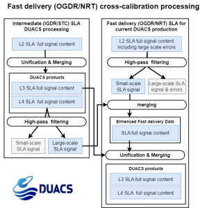
Figure : Overview of the cross-calibration processing for fast delivery (OGDR/NRT) measurements